Teoría BCS

Placa en la
Universidad de Illinois, donde se conmemora el Premio Nobel recibido por John Bardeen gracias al desarrollo de la teoría BCS.
La Teoría BCS (que recibe su nombre de las iniciales de quienes la idearon: John Bardeen, Leon Cooper, y John Robert Schrieffer) fue propuesta en julio de 1957 intentando explicar el fenómeno de la superconductividad. En 1972 los tres recibieron el Premio Nobel de Física gracias a esta teoría.
Esta teoría está considerada como la teoría más importante en el campo de la superconductividad desde el punto de vista microscópico (es decir, tratando de explicar las propiedades de los superconductores a partir de primeros principios). Sin embargo, como se explica más abajo, gran parte de los superconductores siguen sin contar con una explicación satisfactoria.
Contexto histórico
Previamente a la aparición de la teoría BCS, en 1950, Vitaly Ginzburg y Lev Landau presentaron la teoría Ginzburg-Landau, que explicaba varios aspectos de la superconductividad. Sin embargo, las condiciones de la Guerra fría y la poca comunicación que conllevaba entre los miembros de la comunidad científica impidieron que esta teoría influyera sustancialmente el trabajo de Bardeen, Cooper y Schrieffer.
Tras la publicación de la teoría, en 1958, Nikolai Bogoliubov la reafirmó mostrando que la función de onda BCS, que en un principio había sido calculada variacionalmente, se podía obtener también mediante una transformación canónica del hamiltoniano electrónico. Un año más tarde Lev Gor'kov relacionó la teoría BCS con la de Ginzburg-Landau demostrando que esta última es un caso particular de la BCS para temperaturas próximas a la temperatura crítica. El artículo de Gor'kov, publicado en inglésy en ruso, fue a su vez una manera de conciliar ambas teorías a ambos lados del Telón de Acero.
Se considera que en 1964, durante la Conferencia Internacional sobre la Ciencia de la Superconductividad, se alcanzó cierto consenso entre los participantes acerca de la validez de la teoría BCS.
Fundamentos
La atracción de los electrones
La teoría se basa en el hecho de que los portadores de carga no son electrones sino parejas de electrones (conocidas como pares de Cooper). Los electrones habitualmente se repelen debido a que tienen igual carga. Sin embargo, cuando se hallan inmersos en una red cristalina (es decir, la microestructura del material) es posible que la energía entre ellos sea negativa (atractiva) en lugar de positiva (repulsiva), de manera que se creen parejas para minimizar la energía.
Es posible comprender el origen de la atracción entre los electrones gracias a un argumento cualitativo simple. En un metal, los electrones, al tener carga negativa, ejercen una atracción sobre los iones positivos que se encuentran en su vecindad. Estos iones al ser mucho más pesados que los electrones, tienen una inercia mucho mayor. Por esta razón, mientras que un electrón pasa cerca de un conjunto de iones positivos, estos iones no vuelven inmediatamente a su posición de equilibrio original. Ello resulta en un exceso de cargas positivas en el lugar por el que el electrón ha pasado. Un segundo electrón sentirá pues una fuerza atractiva resultado de este exceso de cargas positivas.
Formalmente se suele decir que los electrones interaccionan entre sí mediante fonones, siendo estos una especie de partícula imaginaria que representa la vibración de la red cristalina (generada en este caso por el paso de los electrones).
La banda prohibida superconductora
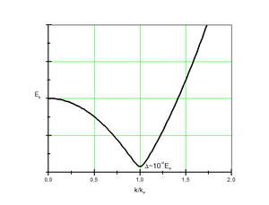
E
k es, en el marco de la teoría BCS, la diferencia de energía entre un sistema en que todos los electrones están en estado superconductor formando pares de Cooper (que sería el estado fundamental), y ese mismo sistema con un único electrón desapareado en el estado
k (que es el primer estado excitado).
Esta especie de "energía de enlace" entre los dos electrones se suele llamar banda prohibida superconductora o, por contagio del inglés, gap superconductor, y se denota Δ. El concepto no está relacionado con la banda prohibida de los semiconductores, salvo en que se comporta de forma parecida.
En un conductor en estado normal (es decir, cuando no es superconductor), es posible excitar un electrón añadiéndole cualquier energía que queramos. Simplemente aumentaremos su energía cinética en igual proporción. Sin embargo, en el caso de un par de Cooper es distinto: si le aplicamos una energía inferior a 2Δ (el doble, debido a que la banda prohibida se toma como energía por electrón), no lograremos excitarlo dado que no romperemos el par. Si la energía es superior a 2Δ, entonces el par se rompe y la energía que le sobre se convierte en energía cinética de los electrones.
Resultados
Fenómenos previos que explica
Algunos de los hechos que son explicados con éxito por esta teoría, y que eran bien conocidos antes de 1957, son los siguientes:
- La existencia de una temperatura crítica, por debajo de la cual el material pasa al estado superconductor.
- La existencia de una discontinuidad en el calor específico al pasar al estado superconductor, con el hecho notable de que, independientemente del material, en el estado superconductor es 2.43 veces mayor que en el normal (para T = Tc).
- El efecto Meissner, descubierto 24 años antes, y por el cual el campo magnético es expulsado del interior del material superconductor, dando lugar a efectos muy populares, como la levitación de imanes.
- El efecto isotópico, descubierto 7 años antes, y según el cual
 , es decir, para distintos isótopos de un elemento superconductor dado, la temperatura crítica es inversamente proporcional a la raíz cuadrada del número másico: cuanto más pesados son los iones positivos, más difícil es alcanzar el estado superconductor. Este efecto jugó un papel muy importante, porque indicó que el estado superconductor tenía algo que ver con la red cristalina, y no tanto con interacciones como el acoplamiento espín-órbita o el acoplamiento espín-espín.
Predicciones explicadas después experimentalmente
En abril de 1957 (tan sólo algunos meses antes de que la teoría BCS saliera a la luz) Richard Feynman, que por entonces se dedicaba al estudio de la superfluidez y la superconductividad, dijo:
No creo que nadie haya calculado nada en física del estado sólido antes de que apareciera el resultado experimental, ¡así que lo único que hemos hecho hasta ahora ha sido predecir lo que ya habíamos observado!
Richard FeynmanSuperfluidity and Superconductivity
Este pensamiento personal (olvidando la Teoría de la Relatividad General) revela la importancia histórica que tuvo la famosa predicción de la teoría BCS:

(donde γ es la constante de Euler-Mascheroni, aproximadamente 0.577).
Lo que dicho de otro modo, viene a significar que si un material tiene una temperatura crítica de 1 K, su banda prohibida será de alrededor de 0.0003 eV. Se realizaron varios experimentos para poner a prueba esta predicción, y se vio que efectivamente en la mayoría de los casos este cociente da un valor cercano a 3.5. La explicación de cómo se llega a este resultado se halla más abajo, en la sección de teoría.
Teoría
Tratamiento mecano-cuántico
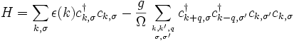
Evidentemente, este argumento cualitativo se justifica por cálculos más rigurosos pues el comportamiento de los electrones y los iones deben describirse por medio de la mecánica cuántica. El tratamiento teórico completo utiliza los métodos de la segunda cuantización, y se basan en el hamiltoniano de Fröhlich:
![H=\sum_{k,\sigma} \epsilon(k) c^\dagger_{k,\sigma} c_{k,\sigma} + \sum_q \hbar \omega_q b^\dagger_q b_q + \frac{1}{\sqrt{\omega}} \sum_{k,q,\sigma} g(k,q) [c^\dagger_{k+q,\sigma} b_q c_{k,\sigma} + c^\dagger_{k+q,\sigma} b^\dagger_{-q} c_{k,\sigma}]](http://upload.wikimedia.org/math/9/5/8/958f59950a31ae5bd74fc39344c5d5a2.png)
donde ck,σ es un operador de aniquilación para un electrón de espín σ, y de momento k, bq es el operador de aniquilación de un fonón de momento q,  y
y  son los operadores de creación correspondientes, y g(k,q) es el elemento de matriz de acoplamiento electrón-fonón. Este término describe la emisión o la absorción de fonones por los electrones. Notar que en este proceso, el momento se conserva.
Por medio de una transformación canónica, se puede eliminar la interacción electrón-fonón del hamiltoniano de Fröhlich para obtener una interacción efectiva entre los electrones. Una aproximación alternativa consiste en utilizar la teoría de perturbaciones de segundo orden en el acoplamiento electrón fonón. En esta aproximación un electrón emite un fonón virtual que es absorbido por otro electrón. Este proceso es la versión cuántica del argumento cualitativo semi-clásico explicado antes. Se encuentra un elemento de matriz para la interacción entre los electrones de la forma:

Este término matricial es en general positivo, lo que corresponde a una interacción repulsiva, pero por  el término se hace negativo lo que corresponde a una interacción atractiva. Estas interacciones atractivas creadas por intercambio de bosones virtuales no se limitan a la física de la materia condensada pues la interacción atractiva entre nucleones en los núcleos atómicos se explica mediante el intercambio de mesones.
Superconductividad en el cero absoluto
Desde el punto de vista teórico, por sencillez, se suele estudiar en primer lugar cómo se comportan los superconductores cuando estamos en el cero absoluto, y en segundo lugar el caso más general, que es cómo se comporta el material a medida que aumentamos la temperatura hasta llegar a la temperatura crítica (y su paso al estado normal).
Así, es posible explicar la relación entre la superconductividad y el efecto isotópico mediante un desarrollo matemático por el cual se llega a:

donde Δ es la banda prohibida y ωD es la frecuencia de Debye. De esta forma, puesto que V0N(0) es una constante que depende del material, vemos que la banda prohibida es proporcional a la energía de excitación  , y puesto que esta a su vez es proporcional a
  , tenemos que la banda prohibida está relacionada con el efecto isotópico.
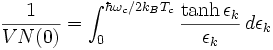
La ecuación de la banda prohibida
Para valores arbitrarios de la temperatura, siempre que esta esté entre 0 y la temperatura crítica, es posible llegar a un importante resultado que se conoce como ecuación de la banda prohibida:

Con esta ecuación, es posible explicar gran número de propiedades de los materiales superconductores, como por ejemplo la ya mencionada relación entre la banda prohibida y la temperatura crítica con un factor 3.53: para ello basta con tener en cuenta que según nos acercamos a la temperatura crítica, el valor de la banda prohibida tiende a cero, de modo que

de modo que

de esta forma, convirtiendo el sumatorio en una integral, nos quedará algo del tipo:
y resolviendo la integral nos quedará que

de donde se puede llegar sin dificultad a la famosa relación ya mencionada.
Limitaciones
Aunque la teoría es notable en cuanto que fue la primera en arrojar luz en este campo, está lejos de ser la teoría definitiva. He aquí algunos ejemplos de ello:
No logra explicar todos los superconductores
Esta teoría explicó bien el comportamiento de ciertos superconductores, conocidos como superconductores convencionales (la mayoría de los cuales son superconductores de tipo I, como el aluminio, el plomo o el mercurio), pero fallaba a la hora de predecir resultados experimentales para los llamados superconductores no convencionales (que suelen ser sustancias más complejas, como aleaciones, cerámicas o fulerenos).
No obstante, hay otra teoría, la teoría Ginzburg-Landau que es de gran ayuda en el estudio de los superconductores no convencionales desde el punto de vista macroscópico (es decir, renunciando a explicar las propiedades rigurosamente a partir de la ecuación de Schrödinger).
Entre estos superconductores no convencionales se encuentran los superconductores de alta temperatura (aquellos que pueden encontrarse en estado superconductor por encima de 77 K), los cuales son famosos porque a día de hoy aún no se ha encontrado una explicación satisfactoria de sus propiedades.
No logra predecir qué materiales serán superconductores
Aun conociendo las propiedades de un material a temperaturas elevadas, la teoría tampoco consigue predecir si éste alcanzará el estado superconductor o no, puesto que se da por sentado que la superconductividad está asociada a la interacción electrón-fonón. Partiendo de esta idea, se supone que una sustancia debería tener más probablididades de ser superconductora a temperaturas relativamente elevadas en los siguientes casos:
- interacción electrón-fonón elevada
- densidad de estados electrónica elevada
- iones de poca masa
Sin embargo, en la práctica, se ha visto que la correlación es muy débil al medir estas propiedades frente al hecho de que la muestra sea superconductora.
source: wikipedia


 .
. . Une paire de Cooper est donc formée de deux électrons de spin opposés et de quasi-impulsions opposées. Plus généralement, une paire de Cooper est formée de deux électrons dans des états reliés l'un à l'autre par renversement du temps. Cette propriété permet de comprendre l'existence de l'effet Meissner dans un supraconducteur. En effet, en présence d'un champ magnétique, la dégénérescence entre états reliés par renversement du temps est levée ce qui réduit l'énergie de liaison des paires de Cooper. Pour garder l'énergie libre gagnée en formant les paires de Cooper, il est avantageux lorsque le champ magnétique est suffisamment faible de l'expulser du supraconducteur. Au delà d'un certain champ magnétique, il est plus avantageux de détruire la supraconductivité soit localement (supraconducteurs de type II) ou globalement (supraconducteurs de type I).
 . Cette propriété est la signature d'un ordre non-diagonal à longue distance. Cet ordre non-diagonal est lié à la brisure de la symétrie de jauge U(1). En effet, si on change les phases des opérateurs de création, (ce qui est une symétrie du Hamiltonien BCS), on change la valeur moyenne du paramètre d'ordre. La fonction d'onde BCS qui a une symétrie plus basse que le Hamiltonien BCS décrit donc une brisure spontanée de symétrie de jauge. Dans la
  comme l'a montré L. P. Gor'kov par des méthodes de fonctions de Green.